Oil immersed transformer Hot-Spot Temperature (HST) models based on IEEE and IEC loading guides
Abstract
This article introduces two models based on the IEEE [1] and IEC [2] loading guides to compute the HST of a transformer winding. The models are solved numerically using arbitrary load and top oil temperature profiles. The results are then compared to highlight relative characteristics of the models.
Introduction
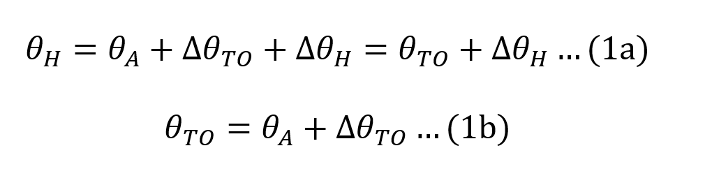
The Transformer Loss of Life (LoL) is based on knowing the HST [3]. It is generally adopted that the HST is given by (1).
Where:
θH is the HST;
θA is the average ambient temperature during the load cycle;
∆θTO is the top oil temperature rise; and
∆θH is hot-spot to top oil temperature rise.
Traditional models [1, 2] estimate the HST based on (1) and require inputs that include: (i) parameters specific to the transformer; and (ii) real-time measurements of ambient temperature, top oil temperature and load current. In recent years transformer manufacturers have included fibre optic sensors (FOS) distributed throughout the windings which conveniently provide an accurate HST measurement leading to a better estimate of the LoL. There are still many transformers in the field that do not incorporate FOS and rely on traditional models for maximising their useful lifespan. This work describes two traditional models for estimating the HST in oil immersed transformers; the models are solved for the HST and compared.
HST models
In our applications, the top oil temperature is provided (measured) and therefore analysis is limited to models that consider only the hot-spot to top oil temperature rise.
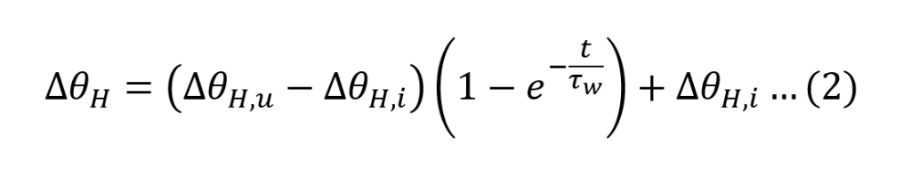
Model 1: The model referred to in Clause 7 [1] as ‘transient heating equation’ is based on work by Kennelly [4] who showed that the winding temperature rise above room temperature is exponential, and Cooney [5] who proposed that the winding temperature rise above top oil and the top oil temperature rise can be treated separately. The model assumes an average ambient temperature of 30°C and step changes in load.
The transient winding HST rise over top oil temperature is given by (2).
Where:
t is the duration of the load;
∆θH is the hot-spot to top oil temperature rise.
∆θH,u is the ultimate winding hottest-spot rise over top oil temperature for the load;
∆θH,i is the initial winding hottest-spot rise over top oil temperature for t=0; and
τW is the winding time constant at the hot-spot location (4.8 minutes [6]).
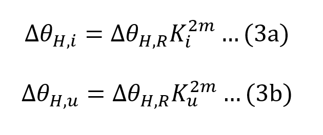
The initial and ultimate HST rises over top oil temperature are given by (3).
Where:
m is an empirically derived exponent to calculate the variation of ∆θH with changes in load (this varies with the type of cooling and equal to 0.8 for ONAN cooling [1];
Ku is the ratio of ultimate load to rated load;
Ki is the ratio of initial load to rated load; and
∆θH,R is the winding hottest-spot rise over top-oil temperature at rated load (typical values range from 20°C to 35°C [6]).
Model 2: The most recent model [2], is based on work by Swift [7] who proposed a thermal model of a power transformer based on heat transfer theory with an equivalent electrical circuit for determining the HST, shown in Figure 1.
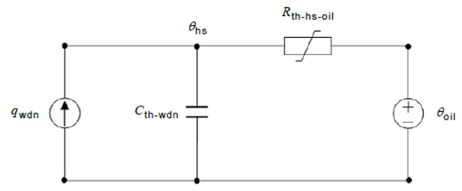
Figure 1: Thermal model of winding-to-oil heat transfer
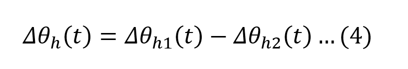
The current source qwdn is the heat generated by the winding losses, Cth-wdn is the thermal capacitance of the winding, Rth-hs-oil is the non-linear winding to oil thermal resistance, and θhs is the HST. Swift’s model is further extended by considering the hot-spot rise dynamic as differences between the fundamental hot-spot rise and the effect of the varying oil flow that influences the HST given by (4).
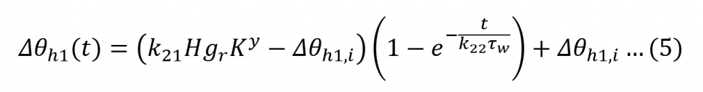
∆θh1 represents the change in the fundamental hot-spot rise given by (5).
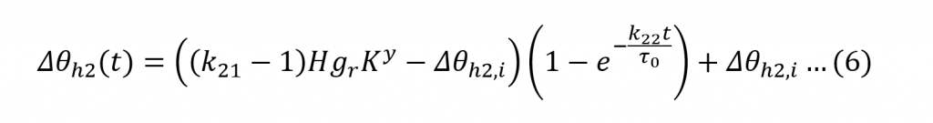
∆θh2 epresents the varying rate of oil flow past the hot-spot, a phenomenon which changes much more slowly and given by (6).
The combined effect of (5) and (6) account for the scenario where a sudden rise in the load current may cause an otherwise unexpectedly high peak in the HST rise, very soon after the sudden load change [2]. Additionally, k21 and k22 are dimensionless parameters and shape (5) and (6) according to Table 1.
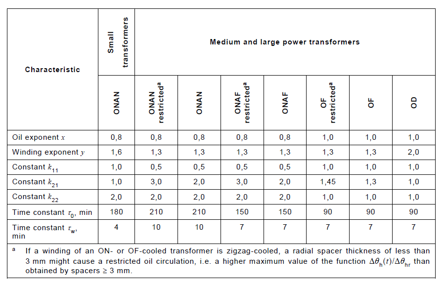
Table 1: Recommended thermal characteristics for exponential equations [2]
Model solutions
In this section equations are solved numerically for various scenarios. The actual time is equal to the time increment, set to 0.0167 minutes, multiplied by the time index shown in the graphs. Distributions of Load Factor (LF) and top oil temperature, shown in Figures 2 and 4, are created for the purpose of highlighting the characteristics of the models.
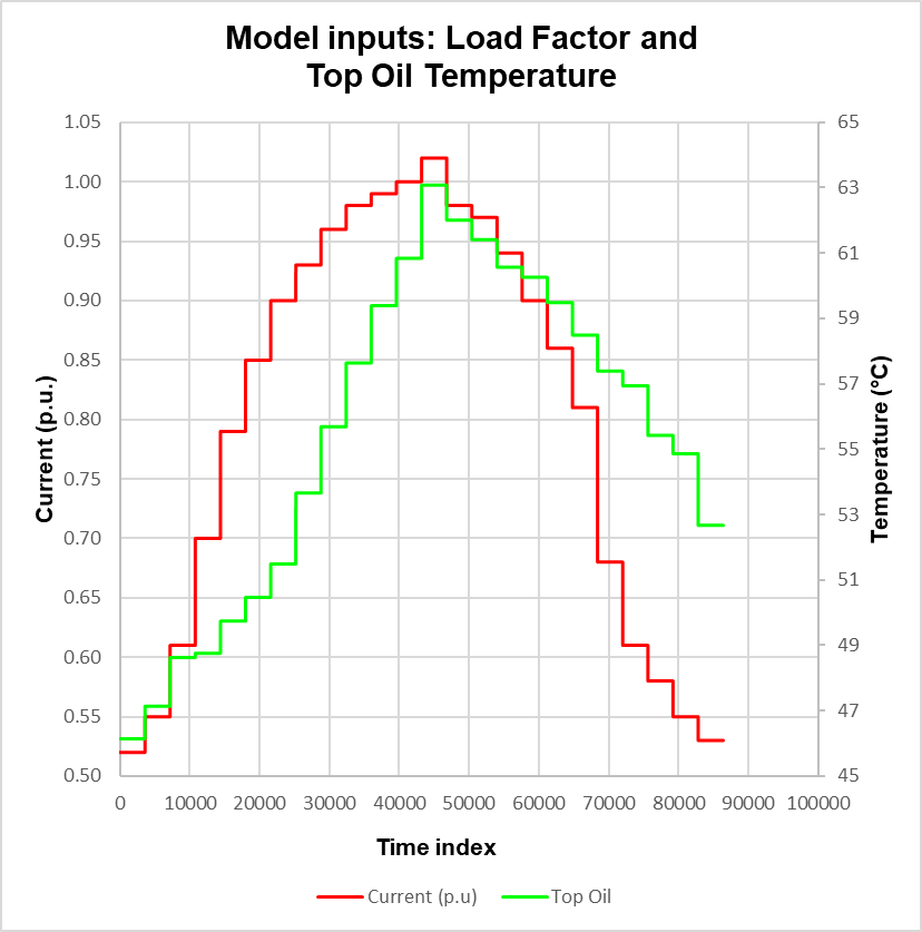
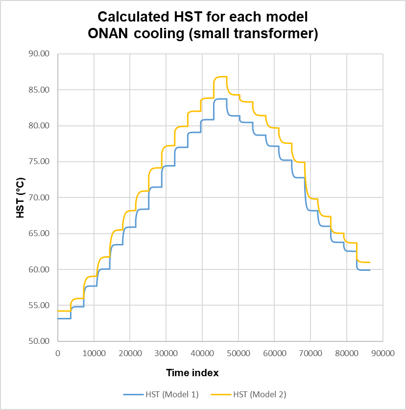
In the case where k21 is set to 1, (6) vanishes because the initial value Δθh2,i is zero leaving only (5). Equations (5) and (2) with (3b) reduce to the same functional form; noting the difference in time constants, τw in (2) and k22τw in (5). Solutions to (1) are shown in Figure 3. As expected, the HST distributions essentially follow the step responses in the top oil temperature profile and also exhibit the exponential growth and decay in accordance with the LF. The maximum variation, Model 2 minus Model 1, is ~3.2°C and occurs at the start of the peak of the LF profile. This is due to the differences in parameters, otherwise both models yield no variation.
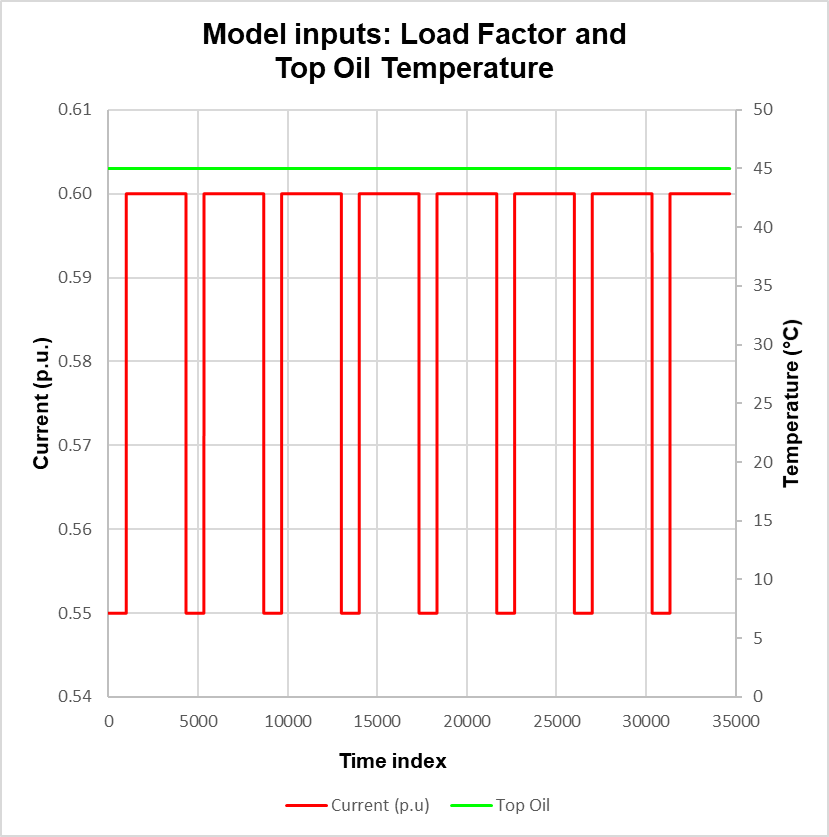
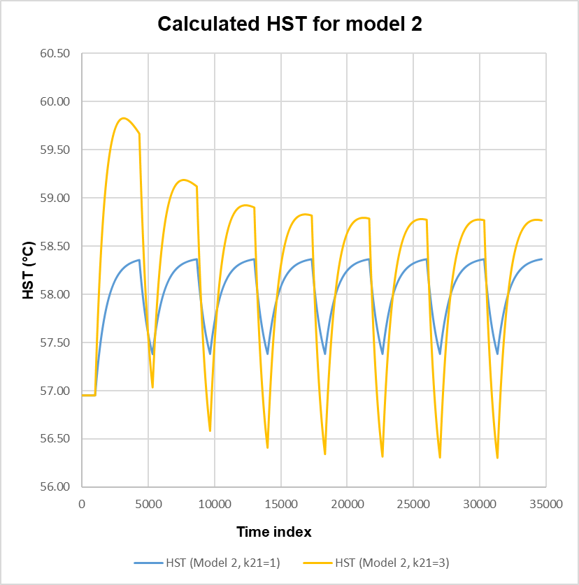
The thermal effect of the oil on the winding HST rise in Model 2 is further investigated by setting k21 to 1 and 3 and by applying the distributions shown in Figure 4. When k21 is set to 1, the effect of oil is not included and the transient behaviour is solely due to the winding constant. Setting k21 to 3 ensures the contribution of the oil time constant in (6) and with (4) now resulting in a subtraction of two first order step responses. The effect is shown in Figure 5, with the response initially exhibiting significant overshoot in the first three excursions and eventually settles to a final value. The effect is due to the inertia of the oil, and is more prevalent in ONANa and ONAFa transformers where oil circulation is restricted, refer to Table 1. The slow decay in the response is due to the oil constant which is ~ 21 times that of the winding constant.
Transformer Monitoring
CHK Power Quality Pty Ltd offers the Miro-F TXM Transformer Monitor and Logger (TxM), an instrument purposely suited for comprehensive monitoring of transformer health and can provide LoL calculations based on the IEC and IEEE Standards.
The TxM includes two temperature sensors which can be software configured to measure the top oil and ambient temperatures. Where the transformer is equipped with multiple winding temperature sensors the TxM, together with the Miro Auxiliary I/0 module (Miro Aux), can utilise these inputs in its LoL calculations.
Setting up and configuring the TXM requires the user to populate a template with relevant transformer ratings and other known parameters specific to the transformer. Alternatively, the user can use default values, provided in the TxM, for parameters that are not readily available on the transformer’s name plate.
The TxM together with the Miro Aux can expand the monitoring to include geomagnetic DC current; dissolved gases such as oxygen; moisture; on load tap changer (OLTC) operation; bushing leakage current; and fan operation. All these parameters can, not only be displayed alongside critical power quality information but also correlated for in depth analysis.
References
[1] “IEEE Guide for loading mineral-oil-immersed transformers and step-voltage regulators”, IEEE Standard C57.91, 2011.
[2] “IEC Power transformers, Part 7: Loading guide for oil-immersed power transformers”, IEC 60076-7, 2018.
[3] “Introduction to Transformer Loss of Life – based on models from IEC and IEEE loading guides”, Transmission and Distribution, Issue 3, June-July 2021, pp. 38-40.
[4] A. E. Kennelly, “The Thermal Time Constants of Dynamo-Electric Machines”, Winter Midwinter Convention of the A.I.E.E Transactions, New York, USA, Feb. 9-13, 1925, pp. 137-154.
[5] W. H. Cooney, ”Predetermination of Self-Cooled Oil-Immersed Transformer Temperatures Before Conditions are Constant”, A.I.E.E Transactions, vol. 44, pp. 611-618, 1925.
[6] “American National Standard guide for loading mineral-oil-immersed power transformers up to and including 100MVA with 55°C or 65°C winding rise”, ANSI/IEEE Standard C57.92, 1981.
[7] G. W. Swift, T. S. Molinski, and W. Lehn, “A Fundamental Approach to Transformer Thermal Modeling – Part 1: Theory and Equivalent Circuit”, IEEE transactions on power delivery, vol. 16, No. 2, pp. 171–177, April 2001.